
Course Info
Course textbooks
Course evaluation
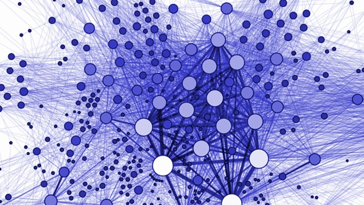
Networks are everywhere!
“Behind each complex system, there is an intricate network that encodes the interactions between the system’s components.” (Barabasi, Network Science)
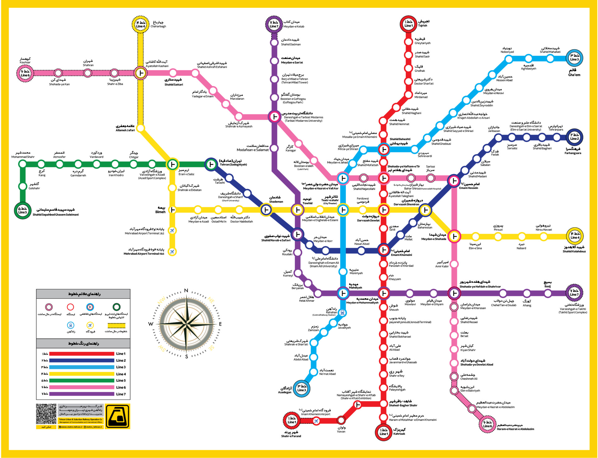
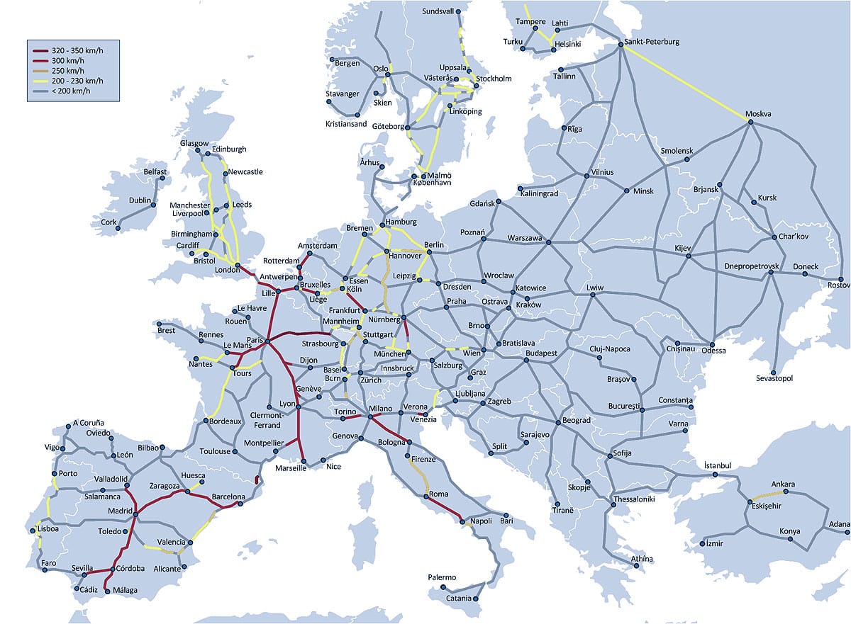
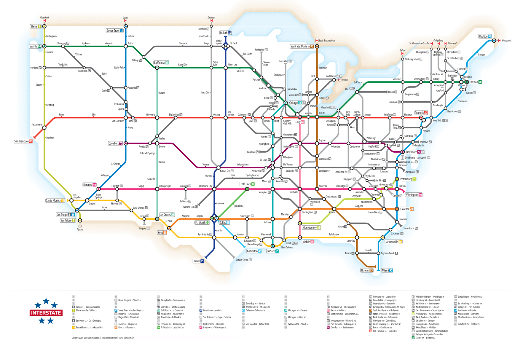
Transportation Networks
Social Networks
Networks in Biology
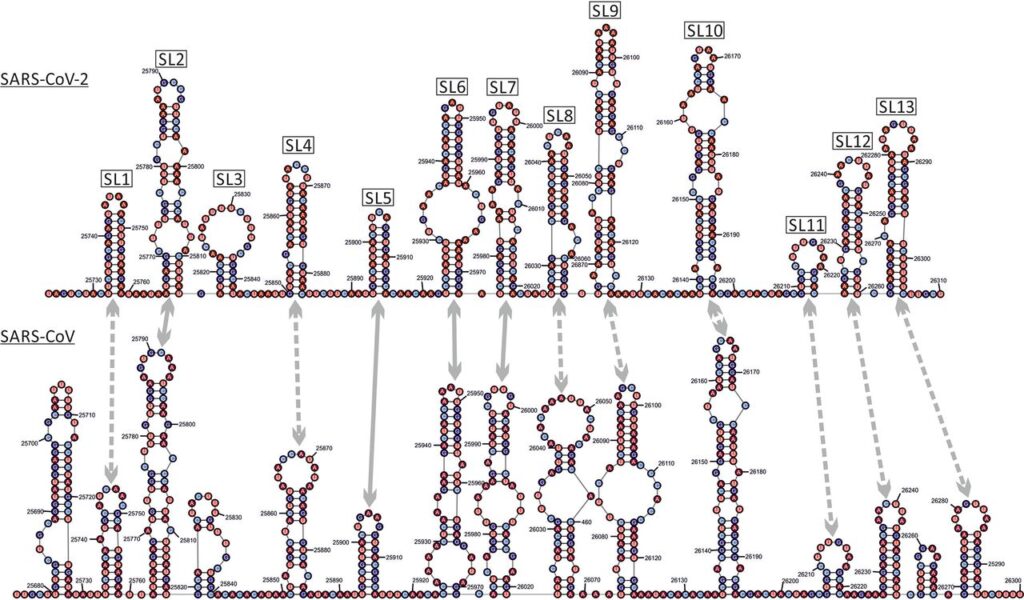
RNA and protein secondary structures
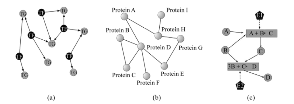
Gene regulatory network
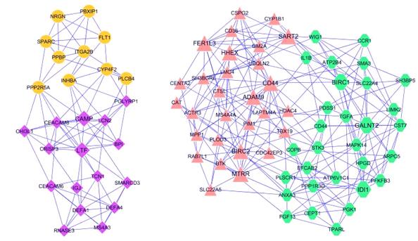 Image credit: www.ese.wustl.edu/nehorai/
Protein-Protein Interaction networks
Metabolic networks
 From left to right: GRN, PPI network and metabolic network. Source: Costa et. al, Complex networks: the key to systems biology
- Albert-László Barabási & Zoltán N. Oltvai, Network biology: understanding the cell’s functional organization, Nature Reviews Genetics, 2004
- Luciano da F. Costa et. al, Complex networks: the key to systems biology
Networks in medicine
Epidemiology
- Danon et al., Networks and the Epidemiology of Infectious Disease, 2011
- D. Balcan, et al., Multiscale mobility networks and the spatial spreading of infectious diseases. PNAS, 2009.
Networks in Neuroscience
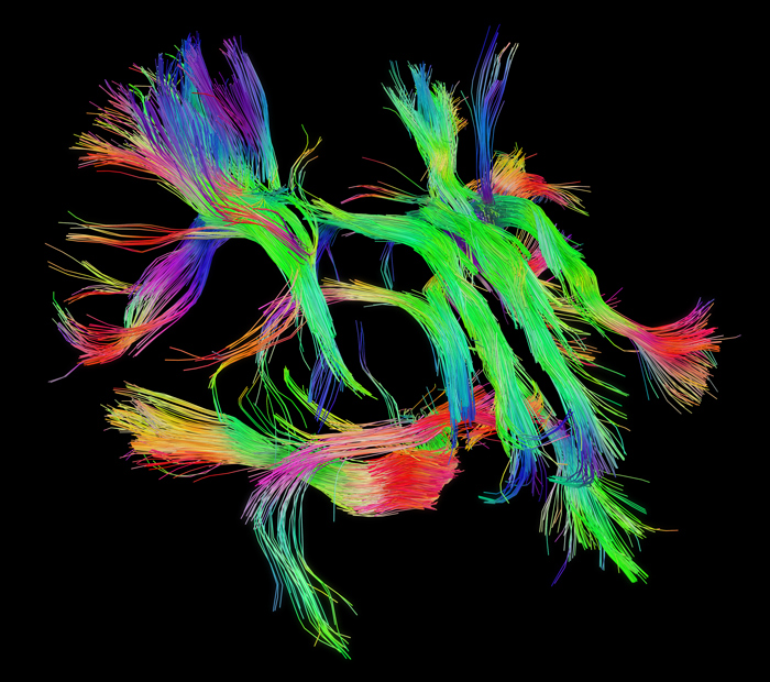 The pathways connecting cortical areas. Source: Human Connectome Project www.humanconnectome.org
Citation networks
Citation network of publications
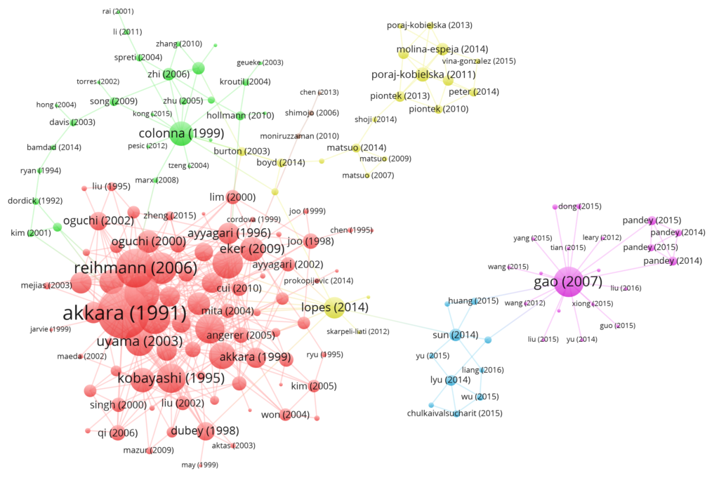 Citation networks are used in bibliometrics and scientometrics.
Collaboration networks
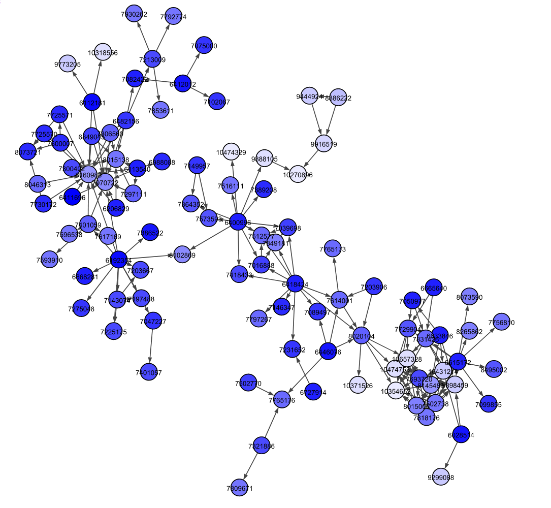
Citation network of patents
- Manajit Chakraborty et al., Patent citation network analysis: A perspective from descriptive statistics and ERGMs
- Triulzi et al., Estimating Technology Performance Improvement Rates by Mining Patent Data, 2020
Web
Networks in Management
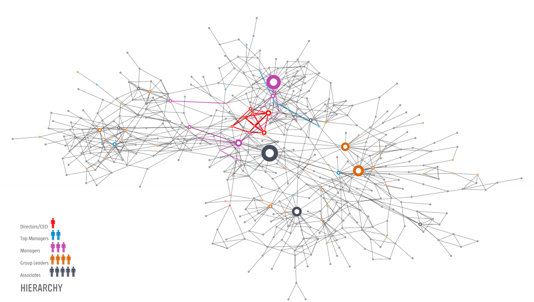 The social network of a Hungarian company. The edges represent “who asks whom for advice”.
Company directors and managers are no among the hubs. The hubs are managers, group leaders and associates, or workers. The biggest hub is an associate. Source: Barabasi, Network Science
The social network of a Hungarian company. The edges represent “who asks whom for advice”.
Company directors and managers are no among the hubs. The hubs are managers, group leaders and associates, or workers. The biggest hub is an associate. Source: Barabasi, Network Science
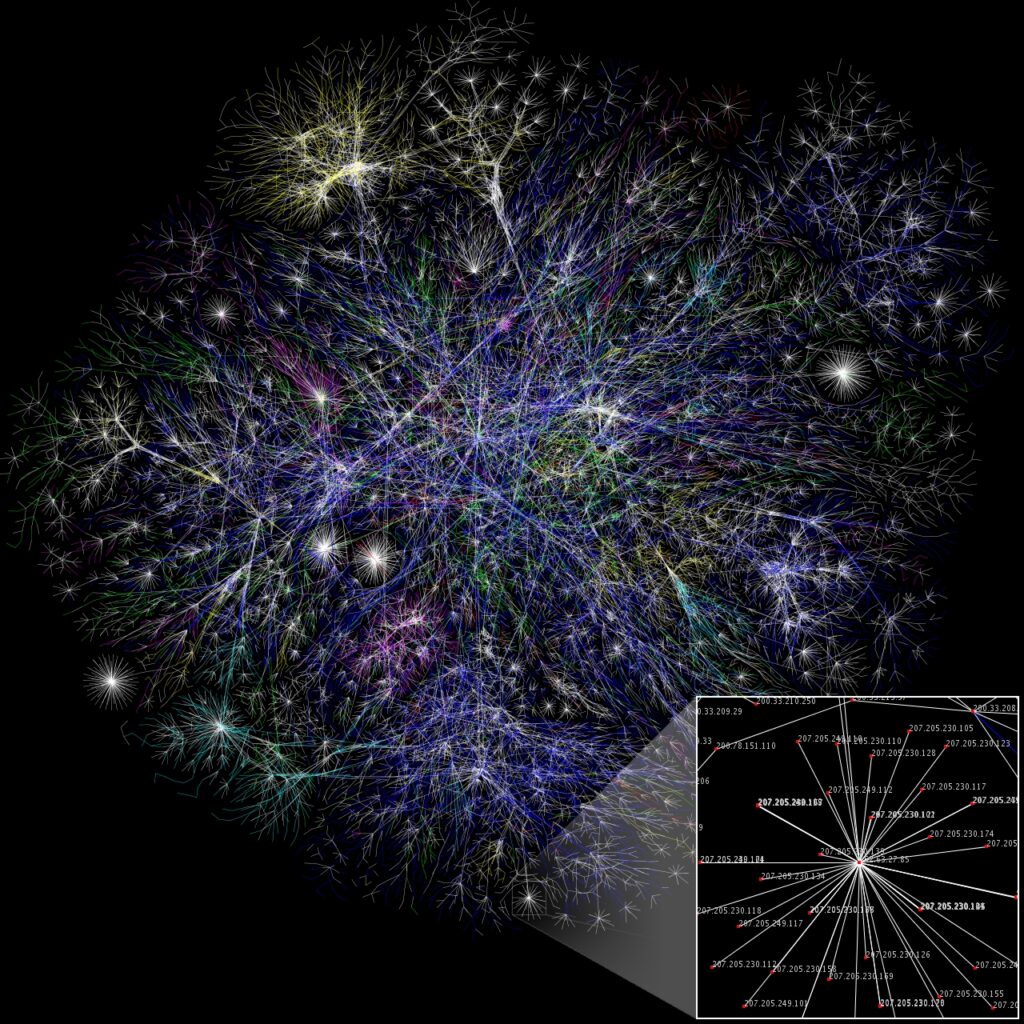
Communication networks
- The internet
The power grid
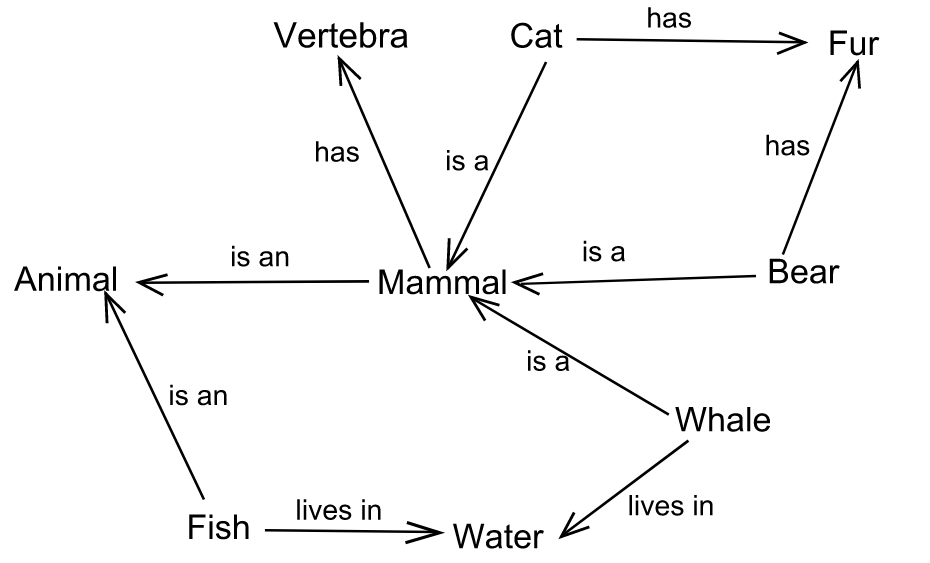
Semantic networks and knowledge graphs
Networks studied in the Network Science book
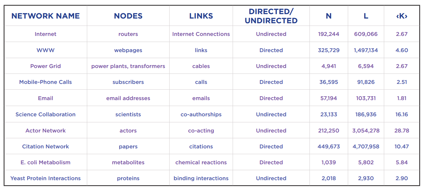 The last three columns are the number of nodes, the number of edges and average degree of nodes.
Network science
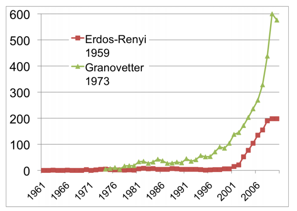 The citation pattern of two of the most highly-cited papers in network theory. Source: Barabasi, Network Science
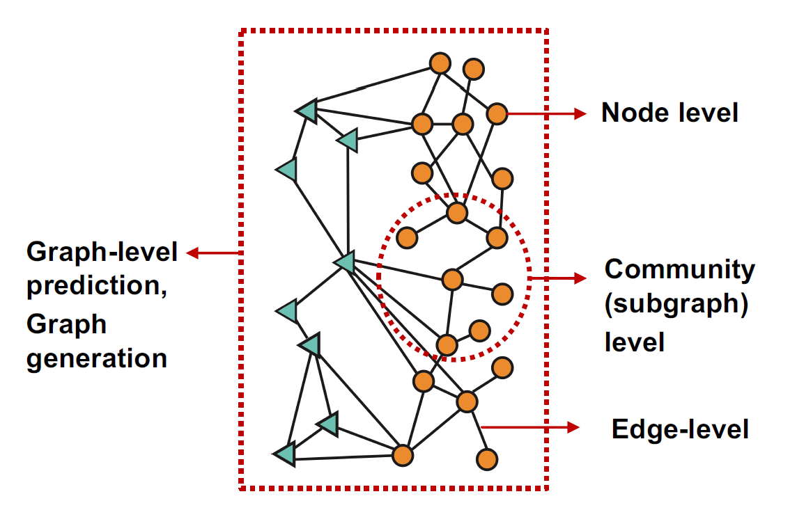 Image source: Jure Leskovec
Syllabus overview
1-Examples of complex networks
2-Graph theory review
3-Network data, network visualization and using Networkx for network analysis
4-Social networks
5-Node level analysis: node centrality and importance
6-Network generative models: random graphs
7-Scale-free networks
8-The Barabasi-Albert model
9-Dynamic networks
10-Network robustness
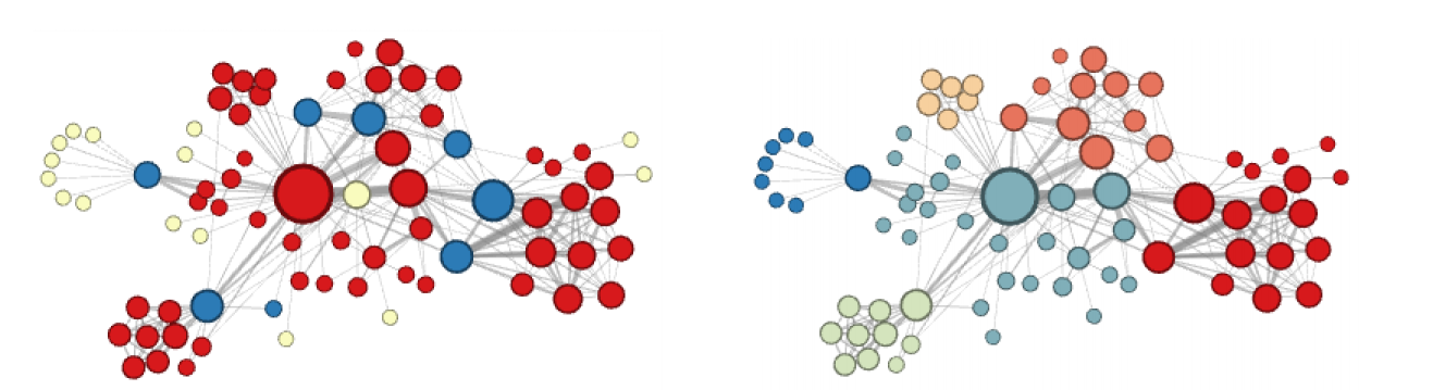
11-Community detection
12-Analysis of the whole network
13-Diffusion in networks
14-Applications of social network analysis
Presentation topics
Statistical mechanics of complex networks
- Albert and Barabasi, Statistical mechanics of complex networks, 2002
- Cimini et al., The statistical physics of real-world networks, Nature, 2019
Mathematical details of random graphs
- Frieze and Kronski, Introduction to Random Graphs, 2024
- Bollobas, Random Graphs, 2001
Topological Data Analysis of networks
- Sizemore et al. The importance of the whole: Topological data analysis for the network neuroscientist
- Taylor et al., Topological data analysis of contagion maps for examining spreading processes on networks, Nature 2015
- Swarup and Rezazadegan, Generating an Agent Taxonomy using Topological Data Analysis, 2019
- Preira, Topological Data Analysis for Network Resilience Quantification, 2021
Spectral graph theory
- Butler, Chung, Spectral Graph Theory
- Graph Representation Learning, section 2.3
- Belkin and Niogy, Laplacian Eigenmaps and Spectral Techniques for Embedding and Clustering
Semantic Networks and knowledge graphs
- Zhou, et al. Derive Word Embeddings From Knowledge Graph
- Ji et al. A Survey on Knowledge Graphs: Representation, Acquisition and Applications
- Graph Representation Learning, Chapter 4
- Wang et al., Knowledge Graph Embedding: A Survey of Approaches and Applications, 2017
- Dai et al., A Survey on Knowledge Graph Embedding: Approaches, Applications and Benchmarks, 2020
Node embedding and node classification (predicting node labels)
- Graph Representation Learning, Chapter 3
- Perozzi, et al., DeepWalk: Online Learning of Social Representations, 2014
- Grover and Leskovec, node2vec: Scalable Feature Learning for Networks
- Leskovec’s course Chapter 3
Graph Neural Networks (GNNs)
- W. Hamilton, Graph Representation Learning, Chapters 5,6
- Jure Leskovec’s Stanford Course:
https://web.stanford.edu/
class/cs224w/ - https://www.pyg.org/
- https://www.dgl.ai/
Theoretical motivation for GNNs
- Graph Representation Learning, Chapter 7
The Weisfeiler-Lehman graph kernel
- Huang, Villar, A Short Tutorial on The Weisfeiler-Lehman Test And Its Variants, 2021
- Shervashidze, Weisfeiler-Lehman Graph Kernels, 2011
- Graph Representation Learning, 2.1.2
Link Prediction
- recommender systems (nodes: products and persons, edges: purchases)
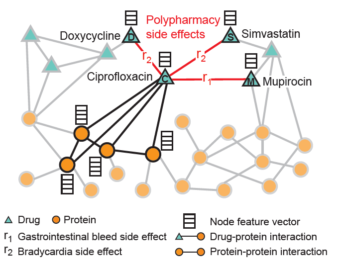
- predicting drug side effects (in the drug-protein interaction network mentioned above).
- Local neighborhood overlap: common Neighbors, Jaccard index, Adamic-Adar index
- Global neighborhood overlap: katz index
- Graph neural networks
- Liben-Nowell, Kleinberg, Link prediction problem for social networks, 2004
- Kumar et al., Link prediction techniques, applications, and performance: A survey, 2020
- Muhan Zhang, Chapter 10 Graph Neural Networks: Link Prediction
- Cleora: A Simple, Strong and Scalable Graph Embedding Scheme
Statistical relational learning
- Khosravi, Bina, Survey on Statistical Relational Learning
- Getoor, Taskar, Introduction to Statistical Relational Learning, MIT Press
Probabilistic Graphical Models
- Zhou, Structure Learning of Probabilistic Graphical Models: A Comprehensive Survey, 2007
Node clustering in graphs
NLP in citation networks
- Brito et al., Network Analysis and Natural Language Processing to Obtain a Landscape of the Scientific Literature on Materials Applications, 2023
Document representation as graphs
- Sonawane, Graph based Representation and Analysis of Text Document: A Survey of Techniques, 2014
- Malliaros, Vazirgiannis, Graph-based Text Representations: Boosting Text Mining, NLP and Information Retrieval with Graphs http://fragkiskosm.github.io/
projects/graph_text_tutorial - Koloski et al., Inducing Document Representations with GRAPH-BASED METHODS: A BLUEPRINT, 2023
Graphs in Natural Language Processing
- Zhou, et al. Derive Word Embeddings From Knowledge Graph
- Nastase, et al., # A survey of graphs in natural language processing, 2015
- Schneider et al., A Decade of Knowledge Graphs in Natural Language Processing: A Survey, 2022
- Wu, et al. Graph Neural Networks for Natural Language Processing: A Survey, 2021
- https://github.com/graph4ai/
graph4nlp
Random walks on networks
- Masuda et al., Random walks and diffusion on networks, 2020
Quantum random walks on networks
- Aharonov et al., Quantum Random Walks on Graphs, 2002
Neo4J and Graph Databases
Deep Generative Graph Models
- Graph Representation Learning, Part III
Spatial Networks
- Barthelemy, Spatial Networks, Physics Reports 2011
Representation learning for temporal networks
- Kazemi et al., Representation Learning for Dynamic Graphs: A Survey, 2020
- Chang et al., Mobility network models of COVID-19 explain inequities and inform reopening, 2020
Traffic prediction
- Derrow-Pinion et al. # ETA Prediction with Graph Neural Networks in Google Maps, 2021
Weather forecasting
- Remi Lam et al., GraphCast: Learning skillful medium-range global weather forecasting, 2023
Stanford Large Network Dataset Collection
http://snap.stanford.edu/data/index.html http://snap.stanford.edu/data/other.htmlNetwork Repository
https://networkrepository.com/index.php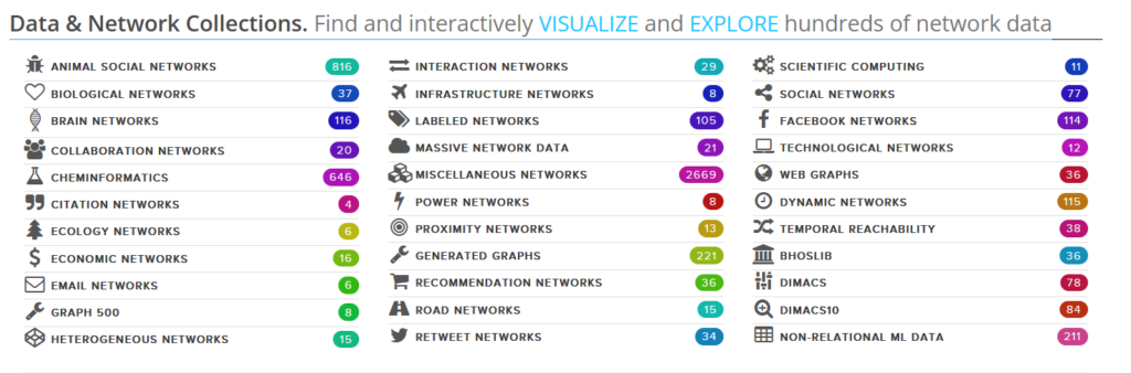
UC Irvine Network Repository
https://networkdata.ics.uci.edu/Social and Communication Networks from Yahoo!
https://webscope.sandbox.yahoo.com/catalog.php?datatype=gNetzschleuder
https://networks.skewed.de/Konect
http://konect.cc/networks/Others
http://math.bu.edu/people/kolaczyk/datasets.html https://public.websites.umich.edu/~mejn/netdata/Network Visualization and Analysis Software
Gephi
Cytoscape
UCINET
for whole-network analysisPajek
Python Libraries
iGraph
- Written in C, available for both R and Python
- Suitable for huge networks with nodes
- Good network visualization tools
- Doesn’t have a very handy API
SNAP.py
https://snap.stanford.edu/snappy/Networkx
Convenient for networks up to 100000 nodes.Introduction to Networkx
Installing Python
Install Miniconda from https://docs.anaconda.com/free/miniconda/miniconda-install.html Then open the Anaconda Prompt and enter pip install networkx jupyter pandas matplotlibCopy Get Visual Studio Code from https://code.visualstudio.com/download Install the Jupyter plugin in VSCode. Optionally install the AI plugin Amazon Code Whisperer.Networkx tutorial
We use this jupyter notebook: https://networkx.org/documentation/stable/tutorial.ipynb Full Networkx reference: https://networkx.org/documentation/hstable/reference/index.htmlStudent presentations from the book Complex Network Analysis with Python
Students make groups of two to present the following chapters:Chapter 3: Constructing a network of Wikipedia pages
Chapter 9: Panama Papers
Chapter 13: Going from Products to Projects
Chapter 16: Building a network of trauma types
Graph Visualization Layouts
Because the networks we study are abstract, there are different ways to draw each network. Topic for a small student presentation!- Tarawneh, et al., A General Introduction To Graph Visualization Techniques
- Ami, Visualization of the Graph Techniques and Different Layouts
Graphs
Reza Rezazadegan
www.dreamintelligent.com
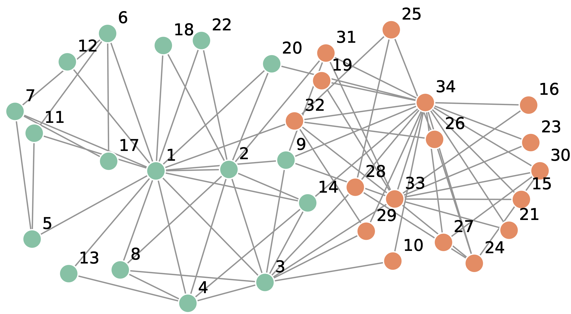
A graph consists of a set of vertices (or nodes) and a set of edges. Each edge is of the form where are vertices of the graph. Such graphs are undirected, meaning that the relations between nodes are symmetric.
A graph can be stored in a computer as a linked list with pointers from nodes to their neighbors.
We denote the number of nodes and links in a network by and respectively.
The degree of a node is the number of edges connected to it. Nodes with relatively high degree are called hubs of the network.
The average degree of a network equal .
The adjacency matrix
After choosing an enumeration of the vertices
, the adjacency matrix of the graph is defined by
if there is an edge between and zero otherwise.
For large networks with thousands or millions of edges, the adjacency matrix will be huge.
Real networks are sparse, meaning that the number of links is proportional to and is much smaller than the possibly number of links i.e. . The neural network of the worm C. elegans, has 297 neurons as nodes and 2,345 synapses as edges.
The adjacency matrix can be stored as a sparse matrix however for large networks it is not efficient to use computationally.
Directed Graphs
In directed networks, relations are asymmetric and thus edges are represented by ordered tuples .
Examples: citation networks, web,…
For directed graphs we have in-degree and out-degree . Of course the sum of the two equals degree of the node: .
We have .
The adjacency matrix of a directed graph is not symmetric:
if there is an edge from towards .
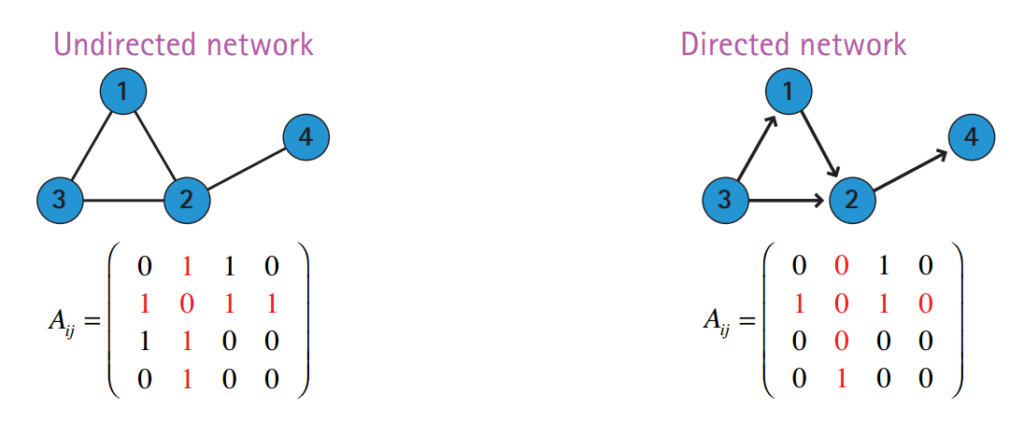
Image credit: Barabasi, Network Science
Every directed graph has an underlying undirected graph which is obtained by symmetrizing the relations.
Weighted Graphs
In the graphs considered so far, all links have the same “value” but in reality, in many networks, the edges have weights which quantifies their role as a link. For example:
- the total length of communication in a mobile network
- the amount of traffic in a communication or transportation network
- the number of clickes on a link between two webpages.
We can encode link weights in the adjacency matrix: .
Paths and connectivity
A path in an undirected network consists of a sequence of nodes such that there is an edge between for each . For directed networks, there must be a directed edge from to . The length of a path is the number of edges in it.
A cycle is a path that starts from a node and goes back to it. A graph is called a tree if it has no cycles.
The distance between two nodes is the minimum length of the paths connecting them. If there is no such a path, the distance is taken to be infinite.
This way a network is a metric space and a topological space.
The diameter of a network is the maximum distance between its nodes.
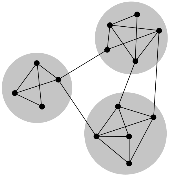
We can define an equivalence relation on graph nodes based on whether there is a path between them. This relation partitions graph nodes into connected components. A graph is connected if it has only one connected component.
The adjacency matrix of a disconnected graph has block-diagonal form.
For directed graphs, distance is measured in the underlying undirected graph. However, even if the underlying undirected graph is connected, there may not be directed paths between pairs of nodes.
For weighted graphs, the length of a path is the sum of its weights. For example in the case of estimating time of arrival, routes with more traffic have a higher weight and can be thought of as being longer.
Relation to adjacency matrix: the number of paths of length 1 from to . Likewise is the number of paths of length 2 between these two vertices. This way, is the number of paths of length from to .
This way, the entries of the matrix equal the number of all paths between pairs of nodes. Note that the above sum equals if all eigenvalues of are and is invertible.
Since even in a small graph, paths can be arbitrarily long, we can introduce an attenuation factor and consider instead. This way longer paths contribute less and the number of paths between to can be thought of as a measure of neighborhood similarity of and . It is called the Katz index of these nodes. In a directed network, Katz index quantifies the influence of on . The sum is a measure of centrality of the node .
Even though above computation is elegant, the adjacency matrix of a large network will be huge. BFS is a better option.
Breath-First Search (BFS)
BFS and DFS are algorithms for finding all the nodes in a graph.
It is a recursive algorithm and uses a queue data structure. Starting from a node u of the graph, BFS labels other nodes by their distance to u. Let F(v) be the function that puts all the unlabeled neighbors of the node v in the queue and labels them with one plus the label of v.
BFS calls F(u) then recursively takes a node v out of the queue and calls F(v) until the queue becomes empty.

Image source: Barabasi, Network Science
def BFS(G, source): # distances from source to nodes dist = {v : Null for v in G} # Create a queue for BFS queue = [] # Mark the source node as # visited and enqueue it queue.append(source) dist[source] = 0 while queue: # Dequeue a vertex from the queue and print it s = queue.pop(0) print(s, end=” “) # Get all adjacent vertices of the dequeued vertex s. # If an adjacent has not been visited, its dist to source is 1+dist[s] and we enqueue it for v in G.nbhs[s]: if dist[v] == None: queue.append(v) dist[v] = dist[s]+1 Copy
Depth-First Search (DFS)
Dijkstra algorithm
BFS algorithm, as is, does not find the shortest path for us. Moreover shortest path finding can be generalized to weighted graphs.
Used for finding best paths in transportation and communication networks e.g. in internet routing.
def dijkstra(graph, source): # Initialize distances and visited set distances = {vertex: float(‘inf’) for vertex in graph} distances[source] = 0 visited = set() while len(visited) < len(graph): current_node = min((node for node in graph if node not in visited), key=distances.get) visited.add(current_node) for (neighbor, weight) in graph[current_node].nbhs(): new_distance = distances[current_node] + weight if new_distance < distances[neighbor]: distances[neighbor] = new_distance return distancesCopy
Graph isomorphism
Two graphs are isomorphic if there is a bijective map such that if then and vice versa.
Induced subgraph
If is a subset of the nodes of the graph, then the subgraph induced by has as vertex set and its edges are the edges of whose nodes are in .
Directed Acyclic Graphs (DAGs) and Topological Decomposition
A directed graph is called acyclic if it has no directed cycles. Citation networks are typically DAGs.
DAGs admit a filtering on their nodes which is called topological decomposition. In this filtering, nodes which in-degree zero are considered level 0. Nodes that receive links from nodes of level 0 are called level 1; nodes that receive links only from nodes of level 1 are considered level 2, and so on. Note that a node receiving links from nodes of levels n and is still considered to be of level n.
There is no link between nodes of each level. Why?
Applications:
- Task scheduling: Ensuring tasks in a project are executed in the correct order.
- Dependency resolution: Installing software packages with dependencies.
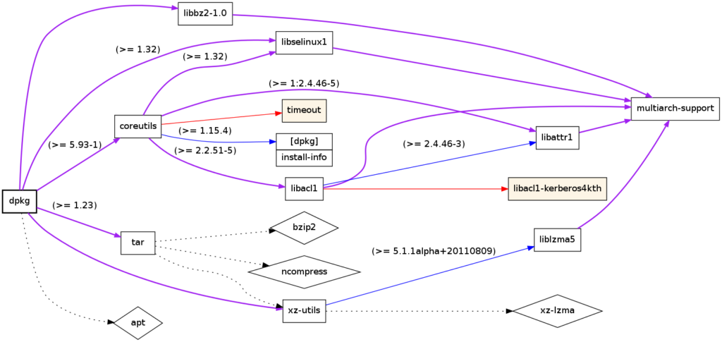
Dependency tree of the Linux package dpkg; produced using debtree
Exercise: Show that the adjacency matrix of a DAG is nilpotent i.e. for some .
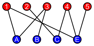
Bipartite graphs
The nodes in a bipartite graph have two types, and there is no edge between the nodes of the same type.
Heterogeneous networks
Such as knowledge graphs, in which nodes and edges can have different types.
Spatial networks
Networks and graphs we considered so far are abstract graphs meaning that there nodes do not have specific locations. However there are many networks whose nodes have spatial locations.
Examples: Mobile antenna towers, transportation networks (such as road networks).
In this course we mainly focus on abstract networks, however see: Barthelemy, Spatial Networks, Physics Reports 2011
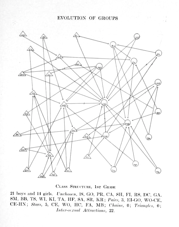
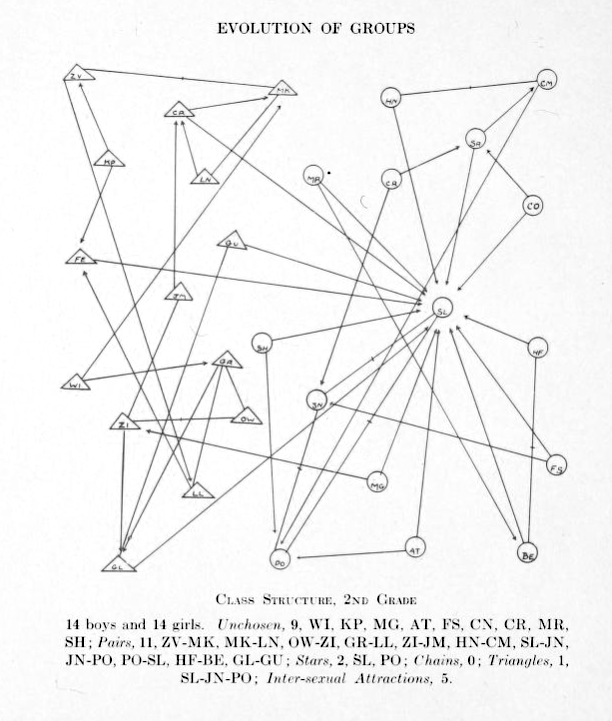
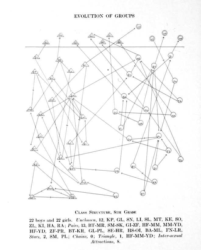 Girls are represented by circles while boys are drawn as triangles.
Source: Jacob Moreno, Who shall survive? A New Approach to the Problem of Human Interrelations, 1934
Girls are represented by circles while boys are drawn as triangles.
Source: Jacob Moreno, Who shall survive? A New Approach to the Problem of Human Interrelations, 1934

Dunbar number
Anthropologist Robin Dunbar realized a relation between the size of the neocortex of primates and the size of their social groups. He proposed that a person cannot handle more than about 150 stable relations at the same time.Giant component
Even if a social network is not connected, it is likely that it has a very large connected component. The giant component is a connected component that contains a “significant” fraction of all the nodes.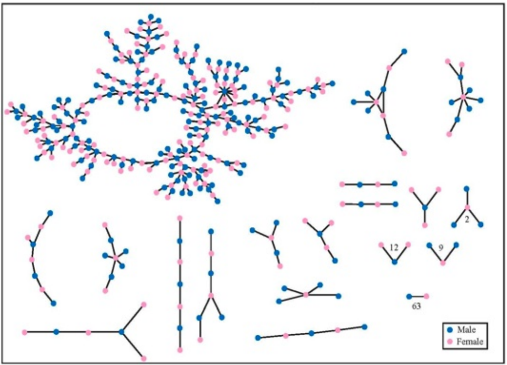 The network of romantic relationships, recorded over a 18 month period, in an American high school. Source: Peter Bearman, James Moody, and Katherine Stovel, American Journal of Sociology, 110(1):44–99, 2004.
Note that there are very few triangles in the network, which (as we will see) means that it has very small clustering coefficient.
If everybody knows an average of 150 people by first name, then we can expect the number of people connected to us to grow exponentially as the hop length (distance) increases.
The network of romantic relationships, recorded over a 18 month period, in an American high school. Source: Peter Bearman, James Moody, and Katherine Stovel, American Journal of Sociology, 110(1):44–99, 2004.
Note that there are very few triangles in the network, which (as we will see) means that it has very small clustering coefficient.
If everybody knows an average of 150 people by first name, then we can expect the number of people connected to us to grow exponentially as the hop length (distance) increases.
Small world phenomenon
Not just large networks have giant connected components, they can have surprisingly short diameters. For example if you have a friend living in a different part of the world, he/she connects you to a whole new network of people. Stanley Milgram mailed 296 letters to randomly chosen addresses in northwestern United States. Recipients were asked to either:- mail the letter to an address in Boston, if they knew the target recepient or,
- send it to someone they knew on the first name basis who was more likely to know the target recepient.
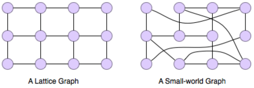 Image Source: Social Network Analysis for Startups, Tsvetovat and Kouznetsov, R’Reilly 2011
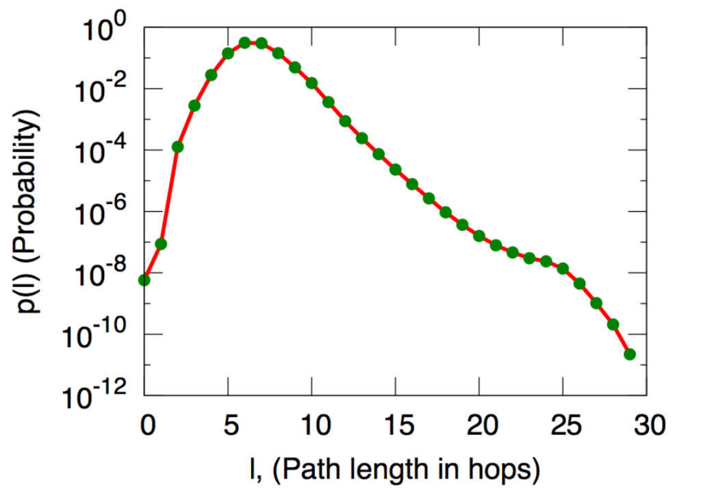 The distribution of distances (more precisely, the average distance to 1000 randomly chosen users) in the network of Microsoft Instant Messager users. An edge in this network means the two users communicated at least once in the one month experiment period. The x axis represents distance and the y axis is the frequency (probability) of that distance among pairs of nodes.
Source: Jure Leskovec and Eric Horvitz, Worldwide buzz: Planetary-scale views on an instant-messaging network. In Proc. 17th International World Wide Web Conference, 2008.
The distribution of distances (more precisely, the average distance to 1000 randomly chosen users) in the network of Microsoft Instant Messager users. An edge in this network means the two users communicated at least once in the one month experiment period. The x axis represents distance and the y axis is the frequency (probability) of that distance among pairs of nodes.
Source: Jure Leskovec and Eric Horvitz, Worldwide buzz: Planetary-scale views on an instant-messaging network. In Proc. 17th International World Wide Web Conference, 2008.
 Collaboration network of mathematicians centered around Paul Erdos. Hand-drawn by Ronald Graham.
https://sites.google.com/oakland.edu/grossman/home/the-erdoes-number-project
Collaboration network of mathematicians centered around Paul Erdos. Hand-drawn by Ronald Graham.
https://sites.google.com/oakland.edu/grossman/home/the-erdoes-number-project
The Watts-Strogatz model for small world networks
Watts-Strogatz model is a model which generated random graphs with small world property. We start with a regular (i.e. all nodes have the same degree) graph in which each node is connected to the nodes near it on the ring. This somehow represents a geographical graph. Then with the probability , each edge is changed into where is chosen uniformly at random and . As nears 1, the graph converges into a random graph. You can experiment with this model here. Image source: Watts, D. J. & Strogatz, S. H. (1998). Collective dynamics of ‘small-world’ networks. Nature 393: 409–10.
Homophily
Homophily: we tend to be similar to our friends. Homophily is a basic phenomenon that affects the structure of social networks.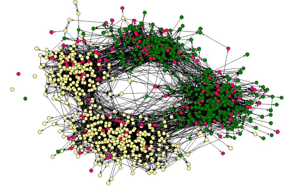 The friendship network in a high school and middle school in America. Node color represents race.
Source: James Moody. Race, school integration, and friendship segregation in America, 2001.
Measuring homophily: Imaging we have two groups of nodes in our network, say male and female. If the probability of being male is and the probability of being female is then if there is no homophily, the probability of existence of a link between a male and a female would be . If the fraction of cross-group edges is significantly less than this (as determined by statistical tests), then we have homophily in the network.
The friendship network in a high school and middle school in America. Node color represents race.
Source: James Moody. Race, school integration, and friendship segregation in America, 2001.
Measuring homophily: Imaging we have two groups of nodes in our network, say male and female. If the probability of being male is and the probability of being female is then if there is no homophily, the probability of existence of a link between a male and a female would be . If the fraction of cross-group edges is significantly less than this (as determined by statistical tests), then we have homophily in the network.
Mechanisms behind homophily:
Selection: A person’s immutable characteristics (race, IQ, age,…) affect the connections and choices they make. Influence: Those to whom we are connected affect our choices. Also called peer pressure. The effect of selection is comparable to, or greater than the effect of social influence.- Denise B. Kandel. Homophily, selection, and socialization in adolescent friendships. American Journal of Sociology, 84(2):427–436, September 1978
- Jere M. Cohen. Sources of peer group homogeneity. Sociology in Education, 50:227–241, October 1977