

Graphs
Reza Rezazadegan
www.dreamintelligent.com
A graph consists of a set of vertices (or nodes) and a set of edges. Each edge is of the form where are vertices of the graph. Such graphs are undirected, meaning that the relations between nodes are symmetric.
A graph can be stored in a computer as a linked list with pointers from nodes to their neighbors.
We denote the number of nodes and links in a network by and respectively.
The degree of a node is the number of edges connected to it. Nodes with relatively high degree are called hubs of the network.
The average degree of a network equal .
The adjacency matrix
After choosing an enumeration of the vertices
, the adjacency matrix of the graph is defined by
if there is an edge between and zero otherwise.
For large networks with thousands or millions of edges, the adjacency matrix will be huge.
Real networks are sparse, meaning that the number of links is proportional to and is much smaller than the possibly number of links i.e. . The neural network of the worm C. elegans, has 297 neurons as nodes and 2,345 synapses as edges.
The adjacency matrix can be stored as a sparse matrix however for large networks it is not efficient to use computationally.
Directed Graphs
In directed networks, relations are asymmetric and thus edges are represented by ordered tuples .
Examples: citation networks, web,…
For directed graphs we have in-degree and out-degree . Of course the sum of the two equals degree of the node: .
We have .
The adjacency matrix of a directed graph is not symmetric:
if there is an edge from towards .
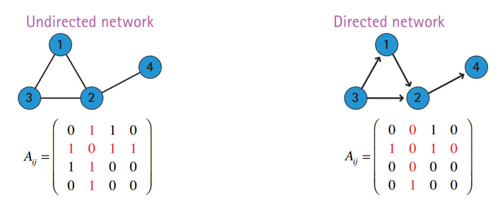
Image credit: Barabasi, Network Science
Every directed graph has an underlying undirected graph which is obtained by symmetrizing the relations.
Weighted Graphs
In the graphs considered so far, all links have the same “value” but in reality, in many networks, the edges have weights which quantifies their role as a link. For example:
- the total length of communication in a mobile network
- the amount of traffic in a communication or transportation network
- the number of clickes on a link between two webpages.
We can encode link weights in the adjacency matrix: .
Paths and connectivity
A path in an undirected network consists of a sequence of nodes such that there is an edge between for each . For directed networks, there must be a directed edge from to . The length of a path is the number of edges in it.
A cycle is a path that starts from a node and goes back to it. A graph is called a tree if it has no cycles.
The distance between two nodes is the minimum length of the paths connecting them. If there is no such a path, the distance is taken to be infinite.
This way a network is a metric space and a topological space.
The diameter of a network is the maximum distance between its nodes.
We can define an equivalence relation on graph nodes based on whether there is a path between them. This relation partitions graph nodes into connected components. A graph is connected if it has only one connected component.
The adjacency matrix of a disconnected graph has block-diagonal form.
For directed graphs, distance is measured in the underlying undirected graph. However, even if the underlying undirected graph is connected, there may not be directed paths between pairs of nodes.
For weighted graphs, the length of a path is the sum of its weights. For example in the case of estimating time of arrival, routes with more traffic have a higher weight and can be thought of as being longer.
Relation to adjacency matrix: the number of paths of length 1 from to . Likewise is the number of paths of length 2 between these two vertices. This way, is the number of paths of length from to .
This way, the entries of the matrix equal the number of all paths between pairs of nodes. Note that the above sum equals if all eigenvalues of are and is invertible.
Since even in a small graph, paths can be arbitrarily long, we can introduce an attenuation factor and consider instead. This way longer paths contribute less and the number of paths between to can be thought of as a measure of neighborhood similarity of and . It is called the Katz index of these nodes. In a directed network, Katz index quantifies the influence of on . The sum is a measure of centrality of the node .
Even though above computation is elegant, the adjacency matrix of a large network will be huge. BFS is a better option.
Breath-First Search (BFS)
BFS and DFS are algorithms for finding all the nodes in a graph.
It is a recursive algorithm and uses a queue data structure. Starting from a node u of the graph, BFS labels other nodes by their distance to u. Let F(v) be the function that puts all the unlabeled neighbors of the node v in the queue and labels them with one plus the label of v.
BFS calls F(u) then recursively takes a node v out of the queue and calls F(v) until the queue becomes empty.

Image source: Barabasi, Network Science
def BFS(G, source): # distances from source to nodes dist = {v : Null for v in G} # Create a queue for BFS queue = [] # Mark the source node as # visited and enqueue it queue.append(source) dist[source] = 0 while queue: # Dequeue a vertex from the queue and print it s = queue.pop(0) print(s, end=” “) # Get all adjacent vertices of the dequeued vertex s. # If an adjacent has not been visited, its dist to source is 1+dist[s] and we enqueue it for v in G.nbhs[s]: if dist[v] == None: queue.append(v) dist[v] = dist[s]+1 Copy
Depth-First Search (DFS)
Dijkstra algorithm
BFS algorithm, as is, does not find the shortest path for us. Moreover shortest path finding can be generalized to weighted graphs.
Used for finding best paths in transportation and communication networks e.g. in internet routing.
def dijkstra(graph, source): # Initialize distances and visited set distances = {vertex: float(‘inf’) for vertex in graph} distances[source] = 0 visited = set() while len(visited) < len(graph): current_node = min((node for node in graph if node not in visited), key=distances.get) visited.add(current_node) for (neighbor, weight) in graph[current_node].nbhs(): new_distance = distances[current_node] + weight if new_distance < distances[neighbor]: distances[neighbor] = new_distance return distancesCopy
Graph isomorphism
Two graphs are isomorphic if there is a bijective map such that if then and vice versa.
Induced subgraph
If is a subset of the nodes of the graph, then the subgraph induced by has as vertex set and its edges are the edges of whose nodes are in .
Directed Acyclic Graphs (DAGs) and Topological Decomposition
A directed graph is called acyclic if it has no directed cycles. Citation networks are typically DAGs.
DAGs admit a filtering on their nodes which is called topological decomposition. In this filtering, nodes which in-degree zero are considered level 0. Nodes that receive links from nodes of level 0 are called level 1; nodes that receive links only from nodes of level 1 are considered level 2, and so on. Note that a node receiving links from nodes of levels n and is still considered to be of level n.
There is no link between nodes of each level. Why?
Applications:
- Task scheduling: Ensuring tasks in a project are executed in the correct order.
- Dependency resolution: Installing software packages with dependencies.
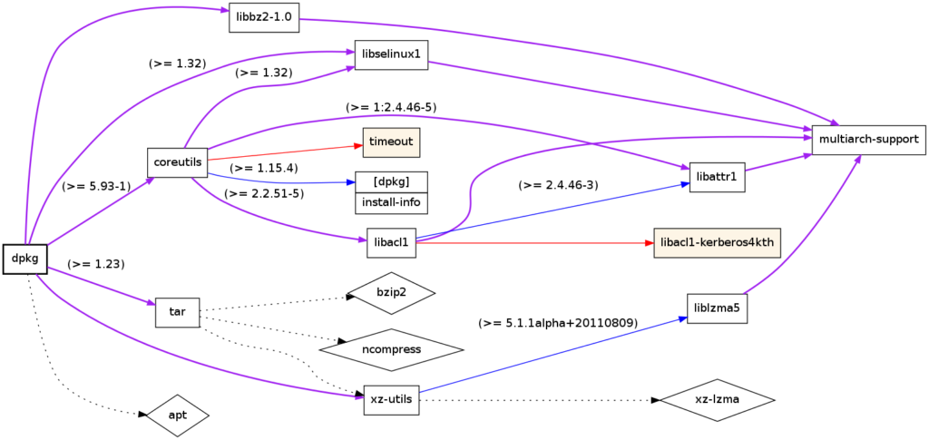
Dependency tree of the Linux package dpkg; produced using debtree
Exercise: Show that the adjacency matrix of a DAG is nilpotent i.e. for some .
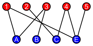
Bipartite graphs
The nodes in a bipartite graph have two types, and there is no edge between the nodes of the same type.
Heterogeneous networks
Such as knowledge graphs, in which nodes and edges can have different types.
Spatial networks
Networks and graphs we considered so far are abstract graphs meaning that there nodes do not have specific locations. However there are many networks whose nodes have spatial locations.
Examples: Mobile antenna towers, transportation networks (such as road networks).
In this course we mainly focus on abstract networks, however see: Barthelemy, Spatial Networks, Physics Reports 2011